| Assignment 4 |
Environmental loads / Environment |
issued 12/2-99 |
Date due 1/3-99 |
| Spectral- estimation |
Disc.: 23/2 & 26/2 |
||
| Solution: 6/3-99 |
|||
This assignment is a discussion on tidal water level data and an example on how we can apply DFT to determine the frequency components of a signal. Apply EXCEL or another IT-tool. In EXCEL you will find the Fourier transform under tools data analysis . Start FFT og follow the instructions. Use 1024 datapoints i.e. 512 hours. NB! The DFT routine i EXCEL defines the Fouriertransform opposite of what Newland does. Therefore you have to check inverse for DFT and do not check inverse for IDFT.
Start EXCEL
a) Look at the table of tidal components below. For a two-week period of observations which components are allowed to include in Fourier analysis?
The answer is: Those marked with an x in the table.
| j |
Symb |
o/h |
Hj cm |
gj o |
|
| 1 |
M2 |
28.9841 |
x |
91.4 |
328 |
| 2 |
S2 |
30 |
x |
32.1 |
5 |
| 3 |
N2 |
28.4397 |
x |
18.2 |
307 |
| K2 |
30.0821 |
- |
|||
| 4 |
K1 |
15.041 |
x |
6.8 |
179 |
| 5 |
O1 |
13.943 |
x |
5.4 |
51 |
| P1 |
14.9589 |
- |
|||
| 6 |
Mf |
1.098 |
x |
2.7 |
187 |
| Mm |
0.0909 |
- |
|||
| Ssa |
0.0802 |
- |
b) Compute
![]() with constants as shown in
the table above for a time period of 3 weeks. Plot the timeseries for a period
of two weeks.
with constants as shown in
the table above for a time period of 3 weeks. Plot the timeseries for a period
of two weeks.
You observe a beat in the signal (amplitude modulation) How long is the beat period and can you explain the causes for it?
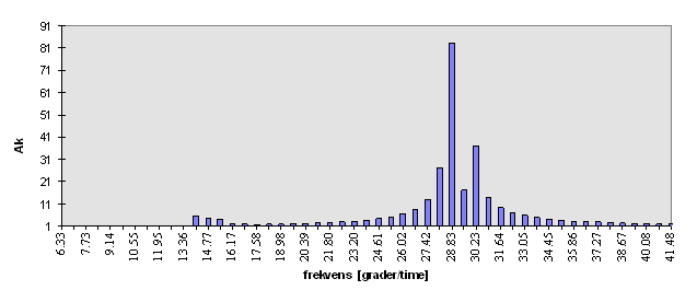
c) Compute DFT of the signal. The result is a series of complex numbers
Xk. 1. Number is for frequency k=0 i.e.
![]() which represents the mean value
of the signal. The next is 1/512 pr hour, next is 2/512 per hour etc. as k/512.
In degrees per hour these become 0, 360/512, 720/512 etc as
which represents the mean value
of the signal. The next is 1/512 pr hour, next is 2/512 per hour etc. as k/512.
In degrees per hour these become 0, 360/512, 720/512 etc as
![]() 360k/512, Thus e.g. the 41.
Frequency is 360*40/512=
360k/512, Thus e.g. the 41.
Frequency is 360*40/512=![]() 28.1o/hour.
28.1o/hour.
Compute ![]() using
2*IMABS(Xk ). Discuss the result. Plot
using
2*IMABS(Xk ). Discuss the result. Plot
.
Ak versus frequency! You should obtain something like this.

Do you find the frequencies from the table above? No! Since the chosen analysis time interval is 512 hours none of the DFT frequencies "hit" the actual frequencies. The variance is therefore spread out on neighbouring components. This phenomenon is often termed as leakage.
d) Lowpass filter the signal by putting high frequency terms equal to zero and perform IDFT. Choose the cut-off frequency equal to 20o/hour. Next, lowpass filter the signal using moving average (cf. Appendix D in the Norwegian compendium) over 2n+1 data points. Use n which gives approx. cut-off frequency of 20o/hour. Perform DFT of this series and compare Ak's with the original with the highest frequencies equal to zero. Comment!.
e) Compute the difference timeseries between the original and the smoothed. You get a highpass filtered timeseries. Perform DFT on this. Are the lowest frequencies contribution to the total variance reduced to next to nothing?
f) Apply the Ak's of the original series and
compute and plot the estimate for the spectral density function (one-sided)
![]() . Write down the formal relation
between Ak og
. Write down the formal relation
between Ak og
![]() giving the unit of the
spectraldensityfunction equal to m2s/rad.
giving the unit of the
spectraldensityfunction equal to m2s/rad.